INSTRUCTIONAL VIDEOS
 Plan of Study
Topographic Mapping Techniques
Traverse and Topographic Mapping
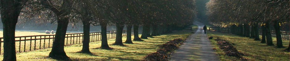
South Louisiana Community College Campus
Lafayette, Louisiana
=P A R T 1=
-1- Plan of study
The links to the videos on this page are for a class taught at the South Louisiana Community College (SLCC), Dept of Civil, Surveying, and Mapping. The videos require about 2 months of study to be able to complete and master.
The plan of study show a student how to process surveying points collected in the field.
Part 1: The first set of 8 videos, processing two coordinate systems
The first set of videos show techniques that were taught in the class room setting. The videos are presented here as reference material.
The first set of points is a traverse connecting a series of rebar monuments placed on the campus of SLCC. These points were processed and given XY coordinates of South Louisiana North American Datum (NAD) 1983 coordinates. This coordinates system is more exact than latitude and longitude using a mercator projection system.
The second set of points are topographical points for a coulee (creek) that runs inside the campus. The coulee itself has cemented sides and bottom. The points are relative points, that is to say without referencing the NAD83 coordinates. The coordinates are simply given a coordinate the first point with an easting of 5,000 and and a north of 7,000. The remaining points are placed in reference to this first point. This procedure is a common one in which a survey crew collects points over a series of days.
The goals then is to import into AutoCAD the first set of traverse points with the absolute NAD83 points and then to import into the same AutoCAD drawing the second set of points with relative set of points. The second set of points are then moved and rotated to match the traverse absolute NAD 83 points.
Part 2:The second set of 8 videos, aerial photos to add topography
This second set of videos are taught online.
This set of videos show how to import a street layer and to import google aerial photos into drawing prepared in the first set of videos. The streets are used to scale the photo.
-2- Drawing Tools: Folio 7 and Pointsin – available on mikeleblanc.net
Folio7 is an AutoCAD plugin (app) developed by the instructor as a set of keyboard commands. Additional information on Folio 7 is available on this website here.
The Folio 7 command are used to draw a wide range of mechanical, architectural, and vicil drawings; but also include a special set of command used in survey plat preparation.
Points is an AutoCAD plugin (app) developed by Tom Haws, a professional engineer in Mesa, Arizona on his website, HawsEDC.com, with a large array of useful surveying data sets, tables, and software tools. Pointsin was modified by Mike LeBlanc to work in tandem with Folio7.
-3- Video #: Download data and review files in folders
This is a demonstration of how to download files used in the sixteen videos.
-3.1- Here is a link to the download page.
-3.2-Screen shots of folders and files as listed on a Mac operating systems.
First set of Folders
01_Documentation
02_Folio7_plug_in
03_Fonts
Second Set of Folders
04_License
05_linetypes
06_plot_pens
07_pointsin
08_profile
09_symbol
10_utilities
11_logo
12_zip
-4- Import traverse pts – absolute coord. (NAD83 XYZ State Plane Coord)
This is a demonstration how to import just the points used in the traverse that we studied in there first part of the course. These points are a traverse on campus with an absolute set of coordinates in Louisiana South, State Plane, North American Datum 1983 (NAD83).
-5- Draw traverse lines clockwise; create polygon; calculate acreage
This is a demonstration how to connect the points in a clockwise manner. After the points are connected with lines, the lines are connected into a polygon. The polygon is measured having 8.8791 acres.If you do not get this answer, then you made a mistake. Please redrawn the polygon and measure it again.
–6- Import topo points – relative coord. (X=5,000; Y= 7,000)
This is aa demonstration of how to import the points marking the location of the two bridges and the edge of the coulee. You will get also points used in the control network that was created from the traverse as mapped in Video 5.
-7- Connect topo points showing center line of coulee (creek)
This is a demonstration of how to create four layers (Bridge_1, Bridge_2, Coule_NS, Coulee_EW) and the connect the points with lines.
–8- Adjust (move and rotate) relative topo pts to absolute traverse coord pts
This is a demonstration how to create a block from the drawing in the previous video by inserting that drawing into the drawing of the original traverse with an absolute set of XY coordinates in NAD83. After being inserted, the drawing is moved and then rotated to align it with the absolute control network.
=P A R T 2=
This is a demonstration how to import streets with the absolute coordinate system into a drawing with the coordinate system. The insertion point needs to be 0,0,0.
-10- Copy Google aerial photos
This is a demonstration how to copy google maps and then import them inside AutoCAD. Once inside, then blocks are created of the original photo along with reference points and survey lines with know bearings.
The photos are selected based on a common set of landmarks both in the photo itself and in the drawing. For example, the photo has both a clearly defined bridge and a street intersection. A survey line connects the bridge centerline and the street intersection. The insertion point of the photo is the bridge when it is blocked.
-11- Import, scale, rotate, and geo-reference Google aerial photos
This is an demonstration how to use the blocks with google photos with marked reference points and survey lines. The blocks are scaled and and then placed to a common landmark found both in the drawing and in the photo. After placing the block, the photo is then rotated to align survey line in both the photo block and the drawing.
This is a demonstration of adding one additional photo into drawing completed in Video 11. How that photo is inserted determines the amount of error found in the resulting topography drawn in the next video.
-12.1 A second photo is inserted into the drawing.
-12.2– The common landmarks in the first photo, and the second photo are the intersection of the centerline of two sides streets (Carl and Shirley) and the centerline of Devalcourt Street. The traverse between these two landmarks is measure by drawing a line along Devalcourt Street’s centerline.
-12.3- The scale factor is calculated by divided the Devalcourt traverse distance in the first photo by the Devalcourt traverse distance in the second photo.
-12.4- The rotation factor is calculated using the bearing of the centerline of the two streets. The bearing in hours (degrees), minutes, and seconds is converted into decimal degrees. The different between there bearing is calculated as the rotation factor.
-12.5- The second photo, the circles marking the landmarks, and the traverse line connecting the two landmarks are blocked.
-12.6- The second photo with landmarks as blocked is inserted with a scale factor at the intersection of the centerline of Shirley and Devalcourt Street.
–12.7- After insertion and scaling, the photo is then rotated using the rotation factor previously calculated.
-12.8- The bridge appears in both in the original survey, the first photo, and the second photo. The centerline of the bridge is measured between the surveyed location and its location in the second photo.
–13- Draw topological features (buildings, parking lots, trees, foot paths and sidewalks, etc.)
This video demonstrates how to outline three buildings (Life Sciences, Ardoin, and Devalcourt) as well as two kinds of parking lots )concrete and limestone) on the southside of the campus. Once polygons are drawn, then different hatch patterns are selected to indicate the kinds of structures.
This is a long video fo 55 minutes showing the implementation of two techniques to create polygons of buildings and parking lots. The first technique simply outlines a continuous polyline to form a polygon around the perimeter of the building. The second techniques uses polyline tangents and connects using the tangents into a polygon with the chamfer command. The two techniques are demonstrated at the beginning of the video. The reminder of the video uses these techniques over and over again. You may not want to view the entire video other than the see last five minutes so as to see which buildings and partings lots were outlined.
-14- Add title sheet; select drawing scale
This video utilizes existing 24 x 36 landscape D size drawings scaled to fit around the area mapped.
–15- Add vicinity map and calculate scale
This is a moderately length video demonstrating how to utilize an existing street map as a vicinity map. Beyond this purpose, the how to use Folio 7 to draw and edit a drawing is demonstrated.
Major arterials and intersecting streets are identified in relation to the campus traverse and associated topography. A circular provides a boundary within which is the campus and the arterials are encapsulated. The remainder of the roadways are erased. The resulting drawing is saved as a separate file and then inserted into the existing traverse and topographic file. The vicinity map is scaled so that it allows the arterials to be named with text. The resulting scale factor in inches on the map being equal to inches in the real world is:
(1/scale factor) x feet per inch = victim map scale factor.
On the example drawn in the video here is the scaling factors used:
existing topo map: 1 inch = 80 feet
scaled vicinity map ratio: .05
(1/.05) x 80 = 20 x 80 ft/in = 1,600 ft/in
-16- Plot map to PDF from model space
The purpose of this video is to demonstrate how to select different colors for line weights of lines and the line weight scale (ltscale command). The color selected for the layers were based on ease of identification. Beyond this purpose, the how to use Folio 7 to draw and edit a drawing is demonstrated so that the color of a layer is modified so the drawing, when plotted, shows a graphic representation of important features by line weights.The hatch patterns are modified as well so that the plotted drawing allows for diffetn parking surfaces to be easily distinguished. The title block and the logo of the client are inserted.
The video is based on other videos used in basic mapping particularly:
Basic CAD Video 03 How set the size of lettering to font points
Basic CAD Video 04 How to create a pen weight table using object colors
Basic CAD Video 05 How to plot to pdf
The resulting drawing converted to a pdf file with corrected line weight is here.
The drawing was corrected according to notes below. The CORRECTED pdf file with collected line weight is here.
Corrections:
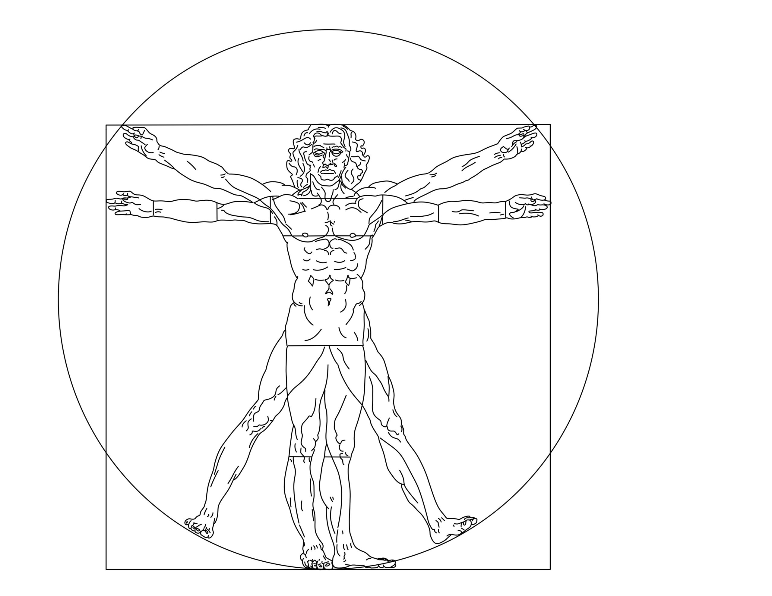
-1- The fictions client’s logo (Vitruvian Man) was drawn by Leonardo da Vinci and NOT Michelangelo. The logo depicts a man in two superimposed positions with his arms and legs apart and inscribed in a circle and square.
-2- The client’s fictions address is in Venice, Italy on San Marco Square. The square was not designed by either Leonardo Di Vinci or Michelangelo; but rather was designed over several centuries as the city grew and the space was modified. It’s true name is Piazza San Marco.